A few years ago, I read an article on pandas’ loc method by Matt Harrison, published on the now-defunct Ponder website. I loved reading it because it showed, in depth, the many ways to use loc. I want to revisit the article and perform in Polars the operations that Matt performed in pandas. Matt also created a chart at the end of the article using pandas’ built-in charting library, which relies on Matplotlib. I’ll recreate two versions of the same chart: one using HvPlot and the other using Glyphx, a new charting library I’m slowly falling in love with.
The dataset
The dataset we’ll be analyzing contains crime data from neighborhoods in Los Angeles. I’ll read the dataset with pandas and store it in a variable called df. The Polars dataframe will be stored in a variable called data.
import pandas as pdurl ="https://data.lacity.org/api/views/2nrs-mtv8/rows.csv?accessType=DOWNLOAD"df = pd.read_csv(url)df.head()
DR_NO
Date Rptd
DATE OCC
TIME OCC
AREA
AREA NAME
Rpt Dist No
Part 1-2
Crm Cd
Crm Cd Desc
...
Status
Status Desc
Crm Cd 1
Crm Cd 2
Crm Cd 3
Crm Cd 4
LOCATION
Cross Street
LAT
LON
0
211507896
04/11/2021 12:00:00 AM
11/07/2020 12:00:00 AM
845
15
N Hollywood
1502
2
354
THEFT OF IDENTITY
...
IC
Invest Cont
354.0
NaN
NaN
NaN
7800 BEEMAN AV
NaN
34.2124
-118.4092
1
201516622
10/21/2020 12:00:00 AM
10/18/2020 12:00:00 AM
1845
15
N Hollywood
1521
1
230
ASSAULT WITH DEADLY WEAPON, AGGRAVATED ASSAULT
...
IC
Invest Cont
230.0
NaN
NaN
NaN
ATOLL AV
N GAULT
34.1993
-118.4203
2
240913563
12/10/2024 12:00:00 AM
10/30/2020 12:00:00 AM
1240
9
Van Nuys
933
2
354
THEFT OF IDENTITY
...
IC
Invest Cont
354.0
NaN
NaN
NaN
14600 SYLVAN ST
NaN
34.1847
-118.4509
3
210704711
12/24/2020 12:00:00 AM
12/24/2020 12:00:00 AM
1310
7
Wilshire
782
1
331
THEFT FROM MOTOR VEHICLE - GRAND ($950.01 AND ...
...
IC
Invest Cont
331.0
NaN
NaN
NaN
6000 COMEY AV
NaN
34.0339
-118.3747
4
201418201
10/03/2020 12:00:00 AM
09/29/2020 12:00:00 AM
1830
14
Pacific
1454
1
420
THEFT FROM MOTOR VEHICLE - PETTY ($950 & UNDER)
...
IC
Invest Cont
420.0
NaN
NaN
NaN
4700 LA VILLA MARINA
NaN
33.9813
-118.4350
5 rows × 28 columns
I’ll read the dataset again with Polars.
import polars as pldata = pl.read_csv(url)data.head()
shape: (5, 28)
DR_NO
Date Rptd
DATE OCC
TIME OCC
AREA
AREA NAME
Rpt Dist No
Part 1-2
Crm Cd
Crm Cd Desc
Mocodes
Vict Age
Vict Sex
Vict Descent
Premis Cd
Premis Desc
Weapon Used Cd
Weapon Desc
Status
Status Desc
Crm Cd 1
Crm Cd 2
Crm Cd 3
Crm Cd 4
LOCATION
Cross Street
LAT
LON
i64
str
str
i64
i64
str
i64
i64
i64
str
str
i64
str
str
i64
str
i64
str
str
str
i64
i64
str
str
str
str
f64
f64
211507896
"04/11/2021 12:00:00 AM"
"11/07/2020 12:00:00 AM"
845
15
"N Hollywood"
1502
2
354
"THEFT OF IDENTITY"
"0377"
31
"M"
"H"
501
"SINGLE FAMILY DWELLING"
null
null
"IC"
"Invest Cont"
354
null
null
null
"7800 BEEMAN …
null
34.2124
-118.4092
201516622
"10/21/2020 12:00:00 AM"
"10/18/2020 12:00:00 AM"
1845
15
"N Hollywood"
1521
1
230
"ASSAULT WITH DEADLY WEAPON, AG…
"0416 0334 2004 1822 1414 0305 …
32
"M"
"H"
102
"SIDEWALK"
200
"KNIFE WITH BLADE 6INCHES OR LE…
"IC"
"Invest Cont"
230
null
null
null
"ATOLL A…
"N GAULT"
34.1993
-118.4203
240913563
"12/10/2024 12:00:00 AM"
"10/30/2020 12:00:00 AM"
1240
9
"Van Nuys"
933
2
354
"THEFT OF IDENTITY"
"0377"
30
"M"
"W"
501
"SINGLE FAMILY DWELLING"
null
null
"IC"
"Invest Cont"
354
null
null
null
"14600 SYLVAN …
null
34.1847
-118.4509
210704711
"12/24/2020 12:00:00 AM"
"12/24/2020 12:00:00 AM"
1310
7
"Wilshire"
782
1
331
"THEFT FROM MOTOR VEHICLE - GRA…
"0344"
47
"F"
"A"
101
"STREET"
null
null
"IC"
"Invest Cont"
331
null
null
null
"6000 COMEY …
null
34.0339
-118.3747
201418201
"10/03/2020 12:00:00 AM"
"09/29/2020 12:00:00 AM"
1830
14
"Pacific"
1454
1
420
"THEFT FROM MOTOR VEHICLE - PET…
"1300 0344 1606 2032"
63
"M"
"H"
103
"ALLEY"
null
null
"IC"
"Invest Cont"
420
null
null
null
"4700 LA VILLA MARINA"
null
33.9813
-118.435
Selecting a row
The loc method in pandas can be used to select specific rows and columns. I’ll select the fifth row in the dataframe.
df.loc[5]
DR_NO                                                240412063
Date Rptd                               12/11/2024 12:00:00 AM
DATE OCC                                11/11/2020 12:00:00 AM
TIME OCC                                                  1210
AREA                                                         4
AREA NAME                                           Hollenbeck
Rpt Dist No                                                429
Part 1-2                                                     2
Crm Cd                                                     354
Crm Cd Desc                                  THEFT OF IDENTITY
Mocodes                                                   0100
Vict Age                                                    35
Vict Sex                                                     M
Vict Descent                                                 B
Premis Cd                                                502.0
Premis Desc       MULTI-UNIT DWELLING (APARTMENT, DUPLEX, ETC)
Weapon Used Cd                                             NaN
Weapon Desc                                                NaN
Status                                                      IC
Status Desc                                        Invest Cont
Crm Cd 1                                                 354.0
Crm Cd 2                                                   NaN
Crm Cd 3                                                   NaN
Crm Cd 4                                                   NaN
LOCATION               5300    CRONUS                       ST
Cross Street                                               NaN
LAT                                                     34.083
LON                                                  -118.1678
Name: 5, dtype: object
Let’s do the same with Polars. I’ll show two ways to select a specific row.
Version 1
(data
 .slice(5, 1)
 )
shape: (1, 28)
DR_NO
Date Rptd
DATE OCC
TIME OCC
AREA
AREA NAME
Rpt Dist No
Part 1-2
Crm Cd
Crm Cd Desc
Mocodes
Vict Age
Vict Sex
Vict Descent
Premis Cd
Premis Desc
Weapon Used Cd
Weapon Desc
Status
Status Desc
Crm Cd 1
Crm Cd 2
Crm Cd 3
Crm Cd 4
LOCATION
Cross Street
LAT
LON
i64
str
str
i64
i64
str
i64
i64
i64
str
str
i64
str
str
i64
str
i64
str
str
str
i64
i64
str
str
str
str
f64
f64
240412063
"12/11/2024 12:00:00 AM"
"11/11/2020 12:00:00 AM"
1210
4
"Hollenbeck"
429
2
354
"THEFT OF IDENTITY"
"0100"
35
"M"
"B"
502
"MULTI-UNIT DWELLING (APARTMENT…
null
null
"IC"
"Invest Cont"
354
null
null
null
"5300 CRONUS …
null
34.083
-118.1678
Version 2
(data
 .gather(5)
 )
shape: (1, 28)
DR_NO
Date Rptd
DATE OCC
TIME OCC
AREA
AREA NAME
Rpt Dist No
Part 1-2
Crm Cd
Crm Cd Desc
Mocodes
Vict Age
Vict Sex
Vict Descent
Premis Cd
Premis Desc
Weapon Used Cd
Weapon Desc
Status
Status Desc
Crm Cd 1
Crm Cd 2
Crm Cd 3
Crm Cd 4
LOCATION
Cross Street
LAT
LON
i64
str
str
i64
i64
str
i64
i64
i64
str
str
i64
str
str
i64
str
i64
str
str
str
i64
i64
str
str
str
str
f64
f64
240412063
"12/11/2024 12:00:00 AM"
"11/11/2020 12:00:00 AM"
1210
4
"Hollenbeck"
429
2
354
"THEFT OF IDENTITY"
"0100"
35
"M"
"B"
502
"MULTI-UNIT DWELLING (APARTMENT…
null
null
"IC"
"Invest Cont"
354
null
null
null
"5300 CRONUS …
null
34.083
-118.1678
Personally, I prefer version 2, but you can use whichever one you like.
Note
You’ve probably noticed that the selected row is displayed differently by the two libraries. Polars displays it horizontally, while pandas displays it vertically.
If we wanted Polars to produce output closer to the pandas output, we could use to_dict to produce a list and then retrieve the first item in that list, which happens to be the dictionary we want.
In Polars, we can display a single column by using the select method.
data.select('Crm Cd 1')
shape: (1_004_894, 1)
Crm Cd 1
i64
354
230
354
331
420
…
510
745
341
230
510
The first thing to note between these two outputs is that when a single column is selected in pandas, the output is a series, unlike in Polars, where the output is always a dataframe regardless of how many columns you select. Another difference is that the pandas output shows an index. Polars dataframes, on the other hand, do not have an index unless you create one.
If we really want the Polars output to be a series as well, we can do it with to_series.
(data
 .select('Crm Cd 1')
 .to_series()
 )
shape: (1_004_894,)
Crm Cd 1
i64
354
230
354
331
420
…
510
745
341
230
510
The two Polars outputs look the same, but they are different types. The way I distinguish between them is by looking at their shape at the top. The dataframe shows both the number of rows and columns: (1004894, 1), while the series only shows the number of rows: (1004894,).
Here’s how we can select two columns and all the rows in the pandas dataframe.
df.loc[:, ['AREA', 'TIME OCC']]
AREA
TIME OCC
0
15
845
1
15
1845
2
9
1240
3
7
1310
4
14
1830
...
...
...
1004889
7
1400
1004890
1
100
1004891
4
2330
1004892
3
1500
1004893
9
2300
1004894 rows × 2 columns
And here’s how to do it the Polars way.
(data
 .select('AREA','TIME OCC')
 )
shape: (1_004_894, 2)
AREA
TIME OCC
i64
i64
15
845
15
1845
9
1240
7
1310
14
1830
…
…
7
1400
1
100
4
2330
3
1500
9
2300
Combine with list of rows and column labels
We can use a list to select the rows we want to return in both pandas and Polars dataframes.
df.loc[[0,1,2], ['AREA', 'TIME OCC']]
AREA
TIME OCC
0
15
845
1
15
1845
2
9
1240
In a Polars dataframe, it is not necessary to use a list to select columns.
Instead of listing the rows or columns we want to select, we can select them over a range. Let’s get the rows from 0 to 2 and the columns from TIME OCC to Part 1-2 in both dataframes.
df.loc[0:2, 'TIME OCC':'Part 1-2']
TIME OCC
AREA
AREA NAME
Rpt Dist No
Part 1-2
0
845
15
N Hollywood
1502
2
1
1845
15
N Hollywood
1521
1
2
1240
9
Van Nuys
933
2
Note
In pandas, range selection using loc is inclusive. Thus, selecting rows from 0 to 2 includes the row at index position 2.
It turns out that in Polars, there is no direct way to select columns over a range by their names. However, we can achieve the same result as in the pandas example using two workarounds. Both require selecting columns by their index positions.
I’ll begin with the one that uses a list comprehension.
We added 1 because, in Polars, index selection is not inclusive. Without it, we would miss the Part 1-2 column in the resulting dataframe.
I would argue that the above method is not idiomatic. List comprehensions are not native to Polars; remember that the library is written in Rust. Here’s the idiomatic approach.
Because loc accepts list comprehensions, we can add logic to customize our row or column selection. The example below pulls out every third row and selects only the columns that contain ‘Crm’ in their names.
df.loc[[Trueif i%3==2elseFalsefor i inrange(len(df))], [Trueif'Crm'in col elseFalsefor col in df.columns]]
Crm Cd
Crm Cd Desc
Crm Cd 1
Crm Cd 2
Crm Cd 3
Crm Cd 4
2
354
THEFT OF IDENTITY
354.0
NaN
NaN
NaN
5
354
THEFT OF IDENTITY
354.0
NaN
NaN
NaN
8
354
THEFT OF IDENTITY
354.0
NaN
NaN
NaN
11
354
THEFT OF IDENTITY
354.0
NaN
NaN
NaN
14
330
BURGLARY FROM VEHICLE
330.0
NaN
NaN
NaN
...
...
...
...
...
...
...
1004879
354
THEFT OF IDENTITY
354.0
NaN
NaN
NaN
1004882
230
ASSAULT WITH DEADLY WEAPON, AGGRAVATED ASSAULT
230.0
NaN
NaN
NaN
1004885
440
THEFT PLAIN - PETTY ($950 & UNDER)
440.0
NaN
NaN
NaN
1004888
341
THEFT-GRAND ($950.01 & OVER)EXCPT,GUNS,FOWL,LI...
341.0
NaN
NaN
NaN
1004891
341
THEFT-GRAND ($950.01 & OVER)EXCPT,GUNS,FOWL,LI...
341.0
NaN
NaN
NaN
334964 rows × 6 columns
We can achieve similar results in Polars by creating an index or by using gather_every. The example below creates an index on the dataframe and performs a modulo calculation on the generated index numbers to get the desired rows. Then we use a regex pattern to select the columns that contain the string ‘Crm’.
Remember that the condition % 3 == 2 keeps rows where the index has a remainder of 2 when divided by 3, i.e., indices 2, 5, 8, 11, and so on. Therefore, the first row selected is index 2, which maps directly to offset=2.
shape: (334_964, 6)
Crm Cd
Crm Cd Desc
Crm Cd 1
Crm Cd 2
Crm Cd 3
Crm Cd 4
i64
str
i64
i64
str
str
354
"THEFT OF IDENTITY"
354
null
null
null
354
"THEFT OF IDENTITY"
354
null
null
null
354
"THEFT OF IDENTITY"
354
null
null
null
354
"THEFT OF IDENTITY"
354
null
null
null
330
"BURGLARY FROM VEHICLE"
330
null
null
null
…
…
…
…
…
…
354
"THEFT OF IDENTITY"
354
null
null
null
230
"ASSAULT WITH DEADLY WEAPON, AG…
230
null
null
null
440
"THEFT PLAIN - PETTY ($950 & UN…
440
null
null
null
341
"THEFT-GRAND ($950.01 & OVER)EX…
341
null
null
null
341
"THEFT-GRAND ($950.01 & OVER)EX…
341
null
null
null
Just to show off how versatile Polars is, I’ll demonstrate other interesting ways to write the code above. I’ll begin with the one that uses the arange function. This also eliminates the need for an index.
Regex patterns are notorious for being difficult to remember. We can avoid them altogether by using special selectors in Polars.
import polars.selectors as cs(data .filter(pl.int_range(pl.len()).mod(3) ==2) .select(cs.contains('Crm')) )
shape: (334_964, 6)
Crm Cd
Crm Cd Desc
Crm Cd 1
Crm Cd 2
Crm Cd 3
Crm Cd 4
i64
str
i64
i64
str
str
354
"THEFT OF IDENTITY"
354
null
null
null
354
"THEFT OF IDENTITY"
354
null
null
null
354
"THEFT OF IDENTITY"
354
null
null
null
354
"THEFT OF IDENTITY"
354
null
null
null
330
"BURGLARY FROM VEHICLE"
330
null
null
null
…
…
…
…
…
…
354
"THEFT OF IDENTITY"
354
null
null
null
230
"ASSAULT WITH DEADLY WEAPON, AG…
230
null
null
null
440
"THEFT PLAIN - PETTY ($950 & UN…
440
null
null
null
341
"THEFT-GRAND ($950.01 & OVER)EX…
341
null
null
null
341
"THEFT-GRAND ($950.01 & OVER)EX…
341
null
null
null
Boolean arrays
Most row filtering in pandas uses boolean masks. Let’s begin with a simple example: filter for rows where AREA NAME is ‘Central’. The code below produces a boolean mask.
We can use this boolean mask in loc to get the desired rows in the dataframe.
df.loc[df['AREA NAME'] =='Central']
DR_NO
Date Rptd
DATE OCC
TIME OCC
AREA
AREA NAME
Rpt Dist No
Part 1-2
Crm Cd
Crm Cd Desc
...
Status
Status Desc
Crm Cd 1
Crm Cd 2
Crm Cd 3
Crm Cd 4
LOCATION
Cross Street
LAT
LON
107
230110144
04/04/2023 12:00:00 AM
07/03/2020 12:00:00 AM
900
1
Central
182
2
354
THEFT OF IDENTITY
...
IC
Invest Cont
354.0
NaN
NaN
NaN
1100 S GRAND AV
NaN
34.0415
-118.2620
563
210118909
10/19/2021 12:00:00 AM
06/02/2020 12:00:00 AM
1605
1
Central
134
1
480
BIKE - STOLEN
...
IC
Invest Cont
480.0
NaN
NaN
NaN
3RD ST
BROADWAY
34.0510
-118.2480
572
210104305
01/08/2021 12:00:00 AM
10/28/2020 12:00:00 AM
1203
1
Central
182
2
668
EMBEZZLEMENT, GRAND THEFT ($950.01 & OVER)
...
IC
Invest Cont
668.0
NaN
NaN
NaN
1200 S FIGUEROA ST
NaN
34.0416
-118.2671
1007
210110076
04/27/2021 12:00:00 AM
07/01/2020 12:00:00 AM
1200
1
Central
155
2
812
CRM AGNST CHLD (13 OR UNDER) (14-15 & SUSP 10 ...
...
AO
Adult Other
812.0
860.0
NaN
NaN
200 E 6TH ST
NaN
34.0448
-118.2474
1708
210104086
01/03/2021 12:00:00 AM
01/03/2020 12:00:00 AM
1510
1
Central
101
2
624
BATTERY - SIMPLE ASSAULT
...
IC
Invest Cont
624.0
NaN
NaN
NaN
900 CENTENNIAL ST
NaN
34.0669
-118.2458
...
...
...
...
...
...
...
...
...
...
...
...
...
...
...
...
...
...
...
...
...
...
1004822
240119704
10/09/2024 12:00:00 AM
10/09/2024 12:00:00 AM
700
1
Central
119
2
888
TRESPASSING
...
IC
Invest Cont
888.0
NaN
NaN
NaN
800 N ALAMEDA ST
NaN
34.0561
-118.2375
1004847
240109835
04/01/2024 12:00:00 AM
04/01/2024 12:00:00 AM
1250
1
Central
152
2
624
BATTERY - SIMPLE ASSAULT
...
IC
Invest Cont
624.0
NaN
NaN
NaN
7TH ST
FLOWER ST
34.0490
-118.2592
1004868
240112635
06/10/2024 12:00:00 AM
06/10/2024 12:00:00 AM
1855
1
Central
138
1
510
VEHICLE - STOLEN
...
IC
Invest Cont
510.0
NaN
NaN
NaN
300 S ALAMEDA ST
NaN
34.0468
-118.2415
1004885
240119644
10/04/2024 12:00:00 AM
09/27/2024 12:00:00 AM
2345
1
Central
142
1
440
THEFT PLAIN - PETTY ($950 & UNDER)
...
IC
Invest Cont
440.0
NaN
NaN
NaN
W 3RD
S GRAND
34.0531
-118.2512
1004890
240104953
01/15/2024 12:00:00 AM
01/15/2024 12:00:00 AM
100
1
Central
101
2
745
VANDALISM - MISDEAMEANOR ($399 OR UNDER)
...
IC
Invest Cont
745.0
NaN
NaN
NaN
1300 W SUNSET BL
NaN
34.0685
-118.2460
69668 rows × 28 columns
By contrast, Polars does not require a boolean mask to perform this filtering operation.
(data .filter(pl.col('AREA NAME') =='Central') )
shape: (69_668, 28)
DR_NO
Date Rptd
DATE OCC
TIME OCC
AREA
AREA NAME
Rpt Dist No
Part 1-2
Crm Cd
Crm Cd Desc
Mocodes
Vict Age
Vict Sex
Vict Descent
Premis Cd
Premis Desc
Weapon Used Cd
Weapon Desc
Status
Status Desc
Crm Cd 1
Crm Cd 2
Crm Cd 3
Crm Cd 4
LOCATION
Cross Street
LAT
LON
i64
str
str
i64
i64
str
i64
i64
i64
str
str
i64
str
str
i64
str
i64
str
str
str
i64
i64
str
str
str
str
f64
f64
230110144
"04/04/2023 12:00:00 AM"
"07/03/2020 12:00:00 AM"
900
1
"Central"
182
2
354
"THEFT OF IDENTITY"
"0930 0929"
25
"M"
"H"
502
"MULTI-UNIT DWELLING (APARTMENT…
null
null
"IC"
"Invest Cont"
354
null
null
null
"1100 S GRAND …
null
34.0415
-118.262
210118909
"10/19/2021 12:00:00 AM"
"06/02/2020 12:00:00 AM"
1605
1
"Central"
134
1
480
"BIKE - STOLEN"
"0344 2032 1822"
35
"M"
"W"
101
"STREET"
null
null
"IC"
"Invest Cont"
480
null
null
null
"3RD S…
"BROADWAY"
34.051
-118.248
210104305
"01/08/2021 12:00:00 AM"
"10/28/2020 12:00:00 AM"
1203
1
"Central"
182
2
668
"EMBEZZLEMENT, GRAND THEFT ($95…
"1501"
0
"M"
"W"
203
"OTHER BUSINESS"
null
null
"IC"
"Invest Cont"
668
null
null
null
"1200 S FIGUEROA …
null
34.0416
-118.2671
210110076
"04/27/2021 12:00:00 AM"
"07/01/2020 12:00:00 AM"
1200
1
"Central"
155
2
812
"CRM AGNST CHLD (13 OR UNDER) (…
null
14
"M"
"H"
501
"SINGLE FAMILY DWELLING"
400
"STRONG-ARM (HANDS, FIST, FEET …
"AO"
"Adult Other"
812
860
null
null
"200 E 6TH …
null
34.0448
-118.2474
210104086
"01/03/2021 12:00:00 AM"
"01/03/2020 12:00:00 AM"
1510
1
"Central"
101
2
624
"BATTERY - SIMPLE ASSAULT"
"1822 0444 1309 0448"
58
"M"
"H"
102
"SIDEWALK"
400
"STRONG-ARM (HANDS, FIST, FEET …
"IC"
"Invest Cont"
624
null
null
null
"900 CENTENNIAL …
null
34.0669
-118.2458
…
…
…
…
…
…
…
…
…
…
…
…
…
…
…
…
…
…
…
…
…
…
…
…
…
…
…
…
240119704
"10/09/2024 12:00:00 AM"
"10/09/2024 12:00:00 AM"
700
1
"Central"
119
2
888
"TRESPASSING"
"0910 2004"
0
"M"
"O"
900
"MTA - RED LINE - UNION STATION"
null
null
"IC"
"Invest Cont"
888
null
null
null
"800 N ALAMEDA …
null
34.0561
-118.2375
240109835
"04/01/2024 12:00:00 AM"
"04/01/2024 12:00:00 AM"
1250
1
"Central"
152
2
624
"BATTERY - SIMPLE ASSAULT"
"2021 2048 1822 0400 0910 0417"
60
"M"
"B"
903
"MTA - RED LINE - 7TH AND METRO…
400
"STRONG-ARM (HANDS, FIST, FEET …
"IC"
"Invest Cont"
624
null
null
null
"7TH S…
"FLOWER S…
34.049
-118.2592
240112635
"06/10/2024 12:00:00 AM"
"06/10/2024 12:00:00 AM"
1855
1
"Central"
138
1
510
"VEHICLE - STOLEN"
null
0
null
null
101
"STREET"
null
null
"IC"
"Invest Cont"
510
null
null
null
"300 S ALAMEDA …
null
34.0468
-118.2415
240119644
"10/04/2024 12:00:00 AM"
"09/27/2024 12:00:00 AM"
2345
1
"Central"
142
1
440
"THEFT PLAIN - PETTY ($950 & UN…
"0344 2014"
42
"F"
"B"
122
"VEHICLE, PASSENGER/TRUCK"
null
null
"IC"
"Invest Cont"
440
null
null
null
"W 3RD"
"S GRAND"
34.0531
-118.2512
240104953
"01/15/2024 12:00:00 AM"
"01/15/2024 12:00:00 AM"
100
1
"Central"
101
2
745
"VANDALISM - MISDEAMEANOR ($399…
"0329 0400 0416"
0
"X"
"X"
503
"HOTEL"
500
"UNKNOWN WEAPON/OTHER WEAPON"
"IC"
"Invest Cont"
745
null
null
null
"1300 W SUNSET …
null
34.0685
-118.246
Now let’s move to a more interesting example. The goal is to select all the columns that have more than the median number of unique values. We’ll calculate the number of unique entries in each column and then find the median value for those counts.
Let’s show the number of unique values in each column of the pandas dataframe.
df.nunique()
DR_NO             1004894
Date Rptd            1870
DATE OCC             1826
TIME OCC             1439
AREA                   21
AREA NAME              21
Rpt Dist No          1210
Part 1-2                2
Crm Cd                140
Crm Cd Desc           140
Mocodes            310912
Vict Age              104
Vict Sex                5
Vict Descent           20
Premis Cd             314
Premis Desc           306
Weapon Used Cd         79
Weapon Desc            79
Status                  6
Status Desc             6
Crm Cd 1              142
Crm Cd 2              126
Crm Cd 3               38
Crm Cd 4                6
LOCATION            66566
Cross Street        10413
LAT                  5426
LON                  4982
dtype: int64
Because the output is displayed vertically, calculating the median is as simple as calling median.
df.nunique().median()
np.float64(140.0)
The calculation is somewhat more involved in Polars. To begin with, the result showing the number of unique values in each column is displayed horizontally as a dataframe.
data.select(pl.all().n_unique())
shape: (1, 28)
DR_NO
Date Rptd
DATE OCC
TIME OCC
AREA
AREA NAME
Rpt Dist No
Part 1-2
Crm Cd
Crm Cd Desc
Mocodes
Vict Age
Vict Sex
Vict Descent
Premis Cd
Premis Desc
Weapon Used Cd
Weapon Desc
Status
Status Desc
Crm Cd 1
Crm Cd 2
Crm Cd 3
Crm Cd 4
LOCATION
Cross Street
LAT
LON
u32
u32
u32
u32
u32
u32
u32
u32
u32
u32
u32
u32
u32
u32
u32
u32
u32
u32
u32
u32
u32
u32
u32
u32
u32
u32
u32
u32
1004894
1870
1826
1439
21
21
1210
2
140
140
310913
104
6
21
315
307
80
80
7
6
143
127
39
7
66566
10414
5426
4982
We can calculate the median value 140.0 by using the transpose method or by using the concat_list function.
Now that we know the median value is 140.0, we can use it to get the desired columns. Here’s how to do it in pandas.
df.loc[:, df.nunique() >140]
DR_NO
Date Rptd
DATE OCC
TIME OCC
Rpt Dist No
Mocodes
Premis Cd
Premis Desc
Crm Cd 1
LOCATION
Cross Street
LAT
LON
0
211507896
04/11/2021 12:00:00 AM
11/07/2020 12:00:00 AM
845
1502
0377
501.0
SINGLE FAMILY DWELLING
354.0
7800 BEEMAN AV
NaN
34.2124
-118.4092
1
201516622
10/21/2020 12:00:00 AM
10/18/2020 12:00:00 AM
1845
1521
0416 0334 2004 1822 1414 0305 0319 0400
102.0
SIDEWALK
230.0
ATOLL AV
N GAULT
34.1993
-118.4203
2
240913563
12/10/2024 12:00:00 AM
10/30/2020 12:00:00 AM
1240
933
0377
501.0
SINGLE FAMILY DWELLING
354.0
14600 SYLVAN ST
NaN
34.1847
-118.4509
3
210704711
12/24/2020 12:00:00 AM
12/24/2020 12:00:00 AM
1310
782
0344
101.0
STREET
331.0
6000 COMEY AV
NaN
34.0339
-118.3747
4
201418201
10/03/2020 12:00:00 AM
09/29/2020 12:00:00 AM
1830
1454
1300 0344 1606 2032
103.0
ALLEY
420.0
4700 LA VILLA MARINA
NaN
33.9813
-118.4350
...
...
...
...
...
...
...
...
...
...
...
...
...
...
1004889
240710284
07/24/2024 12:00:00 AM
07/23/2024 12:00:00 AM
1400
788
NaN
101.0
STREET
510.0
4000 W 23RD ST
NaN
34.0362
-118.3284
1004890
240104953
01/15/2024 12:00:00 AM
01/15/2024 12:00:00 AM
100
101
0329 0400 0416
503.0
HOTEL
745.0
1300 W SUNSET BL
NaN
34.0685
-118.2460
1004891
240410786
10/14/2024 12:00:00 AM
10/11/2024 12:00:00 AM
2330
421
0344
210.0
RESTAURANT/FAST FOOD
341.0
1700 ALBION ST
NaN
34.0675
-118.2240
1004892
240309674
04/24/2024 12:00:00 AM
04/24/2024 12:00:00 AM
1500
358
1822 0334 0416 0445 0449 1202
102.0
SIDEWALK
230.0
FLOWER ST
JEFFERSON BL
34.0215
-118.2868
1004893
240910892
08/13/2024 12:00:00 AM
08/12/2024 12:00:00 AM
2300
914
NaN
108.0
PARKING LOT
510.0
6900 VESPER AV
NaN
34.1961
-118.4510
1004894 rows × 13 columns
And here’s how to do it in Polars.
(data .select(col for col in data.columns if data.select(pl.col(col).n_unique()).item() >140) )
shape: (1_004_894, 13)
DR_NO
Date Rptd
DATE OCC
TIME OCC
Rpt Dist No
Mocodes
Premis Cd
Premis Desc
Crm Cd 1
LOCATION
Cross Street
LAT
LON
i64
str
str
i64
i64
str
i64
str
i64
str
str
f64
f64
211507896
"04/11/2021 12:00:00 AM"
"11/07/2020 12:00:00 AM"
845
1502
"0377"
501
"SINGLE FAMILY DWELLING"
354
"7800 BEEMAN …
null
34.2124
-118.4092
201516622
"10/21/2020 12:00:00 AM"
"10/18/2020 12:00:00 AM"
1845
1521
"0416 0334 2004 1822 1414 0305 …
102
"SIDEWALK"
230
"ATOLL A…
"N GAULT"
34.1993
-118.4203
240913563
"12/10/2024 12:00:00 AM"
"10/30/2020 12:00:00 AM"
1240
933
"0377"
501
"SINGLE FAMILY DWELLING"
354
"14600 SYLVAN …
null
34.1847
-118.4509
210704711
"12/24/2020 12:00:00 AM"
"12/24/2020 12:00:00 AM"
1310
782
"0344"
101
"STREET"
331
"6000 COMEY …
null
34.0339
-118.3747
201418201
"10/03/2020 12:00:00 AM"
"09/29/2020 12:00:00 AM"
1830
1454
"1300 0344 1606 2032"
103
"ALLEY"
420
"4700 LA VILLA MARINA"
null
33.9813
-118.435
…
…
…
…
…
…
…
…
…
…
…
…
…
240710284
"07/24/2024 12:00:00 AM"
"07/23/2024 12:00:00 AM"
1400
788
null
101
"STREET"
510
"4000 W 23RD …
null
34.0362
-118.3284
240104953
"01/15/2024 12:00:00 AM"
"01/15/2024 12:00:00 AM"
100
101
"0329 0400 0416"
503
"HOTEL"
745
"1300 W SUNSET …
null
34.0685
-118.246
240410786
"10/14/2024 12:00:00 AM"
"10/11/2024 12:00:00 AM"
2330
421
"0344"
210
"RESTAURANT/FAST FOOD"
341
"1700 ALBION …
null
34.0675
-118.224
240309674
"04/24/2024 12:00:00 AM"
"04/24/2024 12:00:00 AM"
1500
358
"1822 0334 0416 0445 0449 1202"
102
"SIDEWALK"
230
"FLOWER S…
"JEFFERSON B…
34.0215
-118.2868
240910892
"08/13/2024 12:00:00 AM"
"08/12/2024 12:00:00 AM"
2300
914
null
108
"PARKING LOT"
510
"6900 VESPER …
null
34.1961
-118.451
Closing with a practical example
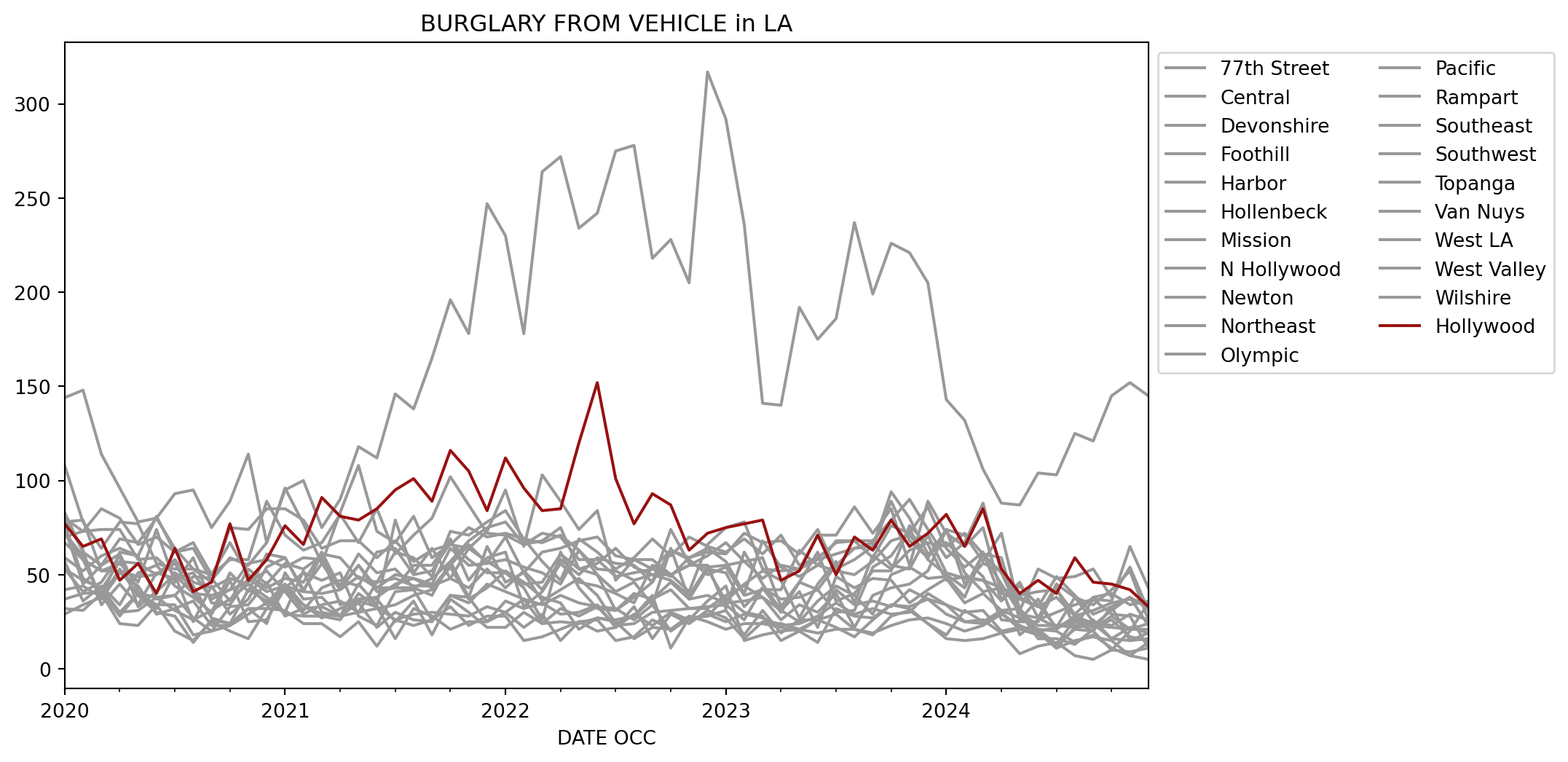
Let’s end with a visualization of the previous analysis. I’ll focus on the Burglary from Vehicle column and plot it over time for the different AREA NAME values. Before we begin creating the charts, I’ll show the dataframe that will be used to create the plot so we know what it looks like.
Move the Hollywood column to the end so that it appears on top of the other columns.
AREA NAME
77th Street
Central
Devonshire
Foothill
Harbor
Hollenbeck
Mission
N Hollywood
Newton
Northeast
...
Pacific
Rampart
Southeast
Southwest
Topanga
Van Nuys
West LA
West Valley
Wilshire
Hollywood
DATE OCC
2020-01-31
75.0
144.0
67.0
37.0
29.0
32.0
53.0
108.0
72.0
80.0
...
70.0
72.0
42.0
53.0
57.0
59.0
83.0
79.0
78.0
77.0
2020-02-29
45.0
148.0
58.0
40.0
34.0
31.0
47.0
78.0
60.0
73.0
...
73.0
58.0
44.0
41.0
36.0
52.0
62.0
63.0
79.0
65.0
2020-03-31
55.0
114.0
52.0
41.0
38.0
40.0
43.0
64.0
37.0
74.0
...
85.0
37.0
38.0
46.0
44.0
60.0
55.0
34.0
52.0
69.0
2020-04-30
61.0
96.0
56.0
28.0
53.0
24.0
30.0
78.0
51.0
74.0
...
80.0
62.0
30.0
60.0
34.0
64.0
69.0
45.0
52.0
47.0
2020-05-31
41.0
78.0
46.0
40.0
39.0
23.0
40.0
77.0
44.0
58.0
...
66.0
60.0
31.0
33.0
51.0
60.0
67.0
34.0
49.0
56.0
2020-06-30
32.0
80.0
74.0
34.0
30.0
34.0
38.0
56.0
29.0
59.0
...
70.0
37.0
38.0
41.0
55.0
81.0
80.0
51.0
50.0
40.0
2020-07-31
51.0
93.0
46.0
34.0
28.0
20.0
39.0
53.0
32.0
50.0
...
62.0
39.0
31.0
50.0
44.0
62.0
64.0
48.0
56.0
64.0
2020-08-31
44.0
95.0
59.0
18.0
14.0
15.0
27.0
53.0
36.0
25.0
...
64.0
49.0
26.0
40.0
38.0
67.0
53.0
51.0
40.0
41.0
2020-09-30
27.0
75.0
35.0
20.0
26.0
25.0
20.0
50.0
23.0
44.0
...
47.0
48.0
31.0
29.0
30.0
50.0
46.0
37.0
39.0
46.0
2020-10-31
24.0
89.0
34.0
23.0
24.0
20.0
33.0
58.0
23.0
29.0
...
59.0
36.0
37.0
47.0
51.0
67.0
75.0
42.0
42.0
77.0
2020-11-30
42.0
114.0
48.0
32.0
32.0
16.0
34.0
58.0
29.0
37.0
...
55.0
53.0
45.0
25.0
41.0
50.0
74.0
46.0
56.0
47.0
2020-12-31
36.0
67.0
41.0
32.0
24.0
32.0
46.0
89.0
35.0
54.0
...
67.0
45.0
38.0
26.0
61.0
43.0
85.0
52.0
58.0
58.0
2021-01-31
30.0
95.0
44.0
42.0
51.0
31.0
28.0
71.0
45.0
59.0
...
96.0
56.0
29.0
43.0
59.0
48.0
85.0
41.0
54.0
76.0
2021-02-28
52.0
100.0
31.0
34.0
37.0
24.0
32.0
63.0
34.0
42.0
...
77.0
53.0
28.0
51.0
41.0
46.0
79.0
29.0
59.0
66.0
2021-03-31
30.0
75.0
43.0
27.0
38.0
24.0
33.0
67.0
29.0
56.0
...
56.0
60.0
28.0
47.0
40.0
62.0
64.0
34.0
58.0
91.0
2021-04-30
28.0
90.0
47.0
32.0
28.0
17.0
28.0
82.0
28.0
42.0
...
83.0
34.0
26.0
51.0
42.0
43.0
68.0
36.0
44.0
81.0
2021-05-31
37.0
118.0
44.0
36.0
35.0
25.0
30.0
67.0
45.0
55.0
...
108.0
37.0
40.0
28.0
49.0
55.0
68.0
30.0
61.0
79.0
2021-06-30
37.0
112.0
62.0
33.0
22.0
12.0
32.0
85.0
34.0
43.0
...
73.0
38.0
33.0
23.0
43.0
41.0
59.0
46.0
51.0
85.0
2021-07-31
25.0
146.0
64.0
16.0
30.0
26.0
34.0
61.0
79.0
50.0
...
67.0
45.0
26.0
41.0
43.0
43.0
68.0
48.0
53.0
95.0
2021-08-31
36.0
138.0
50.0
32.0
26.0
29.0
39.0
71.0
51.0
48.0
...
81.0
48.0
23.0
42.0
43.0
55.0
57.0
44.0
43.0
101.0
2021-09-30
18.0
165.0
52.0
28.0
25.0
30.0
42.0
80.0
64.0
43.0
...
59.0
45.0
26.0
26.0
39.0
55.0
63.0
44.0
48.0
89.0
2021-10-31
37.0
196.0
67.0
21.0
39.0
29.0
54.0
102.0
48.0
55.0
...
66.0
64.0
33.0
39.0
57.0
69.0
66.0
48.0
57.0
116.0
2021-11-30
30.0
178.0
58.0
25.0
38.0
28.0
37.0
87.0
43.0
66.0
...
64.0
55.0
23.0
35.0
38.0
47.0
75.0
64.0
68.0
105.0
2021-12-31
22.0
247.0
51.0
25.0
25.0
33.0
43.0
72.0
53.0
56.0
...
73.0
56.0
28.0
45.0
65.0
59.0
70.0
57.0
75.0
84.0
2022-01-31
22.0
230.0
51.0
30.0
36.0
30.0
52.0
71.0
43.0
70.0
...
95.0
58.0
28.0
41.0
46.0
62.0
72.0
51.0
78.0
112.0
2022-02-28
30.0
178.0
43.0
37.0
32.0
22.0
46.0
66.0
52.0
51.0
...
65.0
54.0
15.0
37.0
51.0
33.0
69.0
45.0
66.0
96.0
2022-03-31
24.0
264.0
26.0
24.0
35.0
29.0
38.0
72.0
42.0
62.0
...
103.0
51.0
17.0
34.0
36.0
41.0
67.0
46.0
68.0
84.0
2022-04-30
32.0
272.0
62.0
25.0
29.0
15.0
35.0
70.0
58.0
64.0
...
89.0
45.0
21.0
39.0
42.0
56.0
71.0
61.0
75.0
85.0
2022-05-31
28.0
234.0
43.0
24.0
30.0
25.0
21.0
58.0
50.0
68.0
...
74.0
63.0
25.0
35.0
48.0
46.0
63.0
53.0
53.0
120.0
2022-06-30
33.0
242.0
32.0
27.0
34.0
26.0
27.0
58.0
59.0
70.0
...
84.0
50.0
20.0
33.0
39.0
44.0
53.0
50.0
56.0
152.0
2022-07-31
32.0
275.0
31.0
25.0
22.0
15.0
26.0
49.0
56.0
60.0
...
47.0
41.0
22.0
23.0
24.0
40.0
52.0
31.0
64.0
101.0
2022-08-31
26.0
278.0
40.0
16.0
29.0
17.0
28.0
51.0
55.0
58.0
...
58.0
46.0
33.0
24.0
28.0
35.0
47.0
38.0
54.0
77.0
2022-09-30
34.0
218.0
37.0
22.0
23.0
26.0
39.0
53.0
46.0
58.0
...
53.0
34.0
16.0
30.0
37.0
55.0
50.0
46.0
50.0
93.0
2022-10-31
20.0
228.0
46.0
21.0
30.0
21.0
11.0
49.0
63.0
50.0
...
63.0
64.0
29.0
31.0
42.0
50.0
50.0
74.0
47.0
87.0
2022-11-30
27.0
205.0
37.0
26.0
26.0
28.0
27.0
59.0
58.0
41.0
...
59.0
37.0
24.0
32.0
32.0
55.0
55.0
56.0
39.0
63.0
2022-12-31
28.0
317.0
39.0
36.0
29.0
25.0
28.0
64.0
50.0
66.0
...
62.0
53.0
31.0
32.0
33.0
55.0
60.0
53.0
54.0
72.0
2023-01-31
31.0
292.0
35.0
44.0
25.0
21.0
38.0
57.0
54.0
75.0
...
61.0
51.0
27.0
39.0
34.0
32.0
67.0
36.0
55.0
75.0
2023-02-28
18.0
236.0
36.0
15.0
29.0
24.0
30.0
40.0
39.0
78.0
...
72.0
33.0
16.0
44.0
26.0
62.0
57.0
45.0
57.0
77.0
2023-03-31
31.0
141.0
38.0
18.0
27.0
24.0
28.0
68.0
42.0
53.0
...
67.0
43.0
25.0
38.0
43.0
45.0
59.0
52.0
48.0
79.0
2023-04-30
19.0
140.0
26.0
20.0
23.0
22.0
15.0
54.0
42.0
52.0
...
68.0
30.0
24.0
31.0
37.0
31.0
33.0
47.0
55.0
47.0
2023-05-31
26.0
192.0
34.0
21.0
24.0
20.0
20.0
49.0
63.0
53.0
...
61.0
46.0
21.0
41.0
38.0
25.0
46.0
27.0
53.0
52.0
2023-06-30
26.0
175.0
30.0
19.0
28.0
26.0
14.0
55.0
55.0
58.0
...
74.0
62.0
26.0
22.0
42.0
36.0
42.0
45.0
71.0
71.0
2023-07-31
42.0
186.0
40.0
21.0
35.0
22.0
32.0
52.0
68.0
61.0
...
53.0
36.0
29.0
49.0
30.0
44.0
55.0
57.0
71.0
50.0
2023-08-31
34.0
237.0
22.0
21.0
29.0
17.0
28.0
50.0
68.0
64.0
...
58.0
40.0
21.0
43.0
31.0
39.0
64.0
35.0
86.0
70.0
2023-09-30
36.0
199.0
39.0
19.0
32.0
26.0
27.0
57.0
59.0
67.0
...
65.0
52.0
18.0
48.0
54.0
29.0
65.0
60.0
72.0
63.0
2023-10-31
33.0
226.0
43.0
23.0
29.0
34.0
34.0
68.0
76.0
55.0
...
89.0
52.0
28.0
47.0
60.0
50.0
94.0
53.0
85.0
79.0
2023-11-30
42.0
221.0
45.0
26.0
30.0
32.0
33.0
71.0
72.0
53.0
...
68.0
76.0
31.0
35.0
74.0
54.0
80.0
63.0
55.0
65.0
2023-12-31
37.0
205.0
52.0
27.0
40.0
24.0
37.0
59.0
86.0
71.0
...
59.0
66.0
24.0
42.0
58.0
48.0
61.0
67.0
89.0
72.0
2024-01-31
34.0
143.0
74.0
24.0
34.0
18.0
29.0
74.0
64.0
51.0
...
74.0
47.0
16.0
48.0
50.0
49.0
67.0
65.0
72.0
82.0
2024-02-29
30.0
132.0
45.0
20.0
25.0
31.0
25.0
51.0
54.0
48.0
...
71.0
49.0
15.0
35.0
43.0
38.0
58.0
72.0
65.0
65.0
2024-03-31
31.0
106.0
56.0
23.0
26.0
25.0
24.0
41.0
62.0
47.0
...
57.0
47.0
16.0
40.0
61.0
61.0
49.0
61.0
75.0
85.0
2024-04-30
20.0
88.0
52.0
29.0
19.0
31.0
30.0
43.0
37.0
36.0
...
72.0
43.0
19.0
31.0
59.0
45.0
26.0
51.0
40.0
53.0
2024-05-31
22.0
87.0
29.0
23.0
21.0
27.0
21.0
38.0
44.0
46.0
...
31.0
18.0
8.0
32.0
26.0
30.0
25.0
30.0
37.0
40.0
2024-06-30
21.0
104.0
27.0
19.0
18.0
21.0
21.0
33.0
34.0
27.0
...
53.0
26.0
12.0
20.0
37.0
16.0
25.0
23.0
33.0
47.0
2024-07-31
11.0
103.0
22.0
11.0
13.0
20.0
13.0
38.0
22.0
45.0
...
48.0
30.0
14.0
22.0
21.0
16.0
43.0
23.0
49.0
40.0
2024-08-31
22.0
125.0
25.0
15.0
21.0
14.0
26.0
28.0
38.0
38.0
...
49.0
34.0
7.0
27.0
28.0
13.0
22.0
22.0
39.0
59.0
2024-09-30
26.0
121.0
20.0
17.0
20.0
18.0
22.0
31.0
25.0
34.0
...
53.0
37.0
5.0
23.0
24.0
21.0
37.0
23.0
29.0
46.0
2024-10-31
16.0
145.0
33.0
15.0
10.0
11.0
26.0
35.0
23.0
42.0
...
38.0
36.0
10.0
22.0
16.0
28.0
29.0
31.0
33.0
45.0
2024-11-30
15.0
152.0
15.0
7.0
20.0
7.0
17.0
37.0
29.0
52.0
...
54.0
65.0
9.0
21.0
22.0
21.0
28.0
38.0
38.0
42.0
2024-12-31
16.0
145.0
19.0
5.0
35.0
14.0
15.0
35.0
26.0
26.0
...
31.0
43.0
11.0
24.0
19.0
21.0
11.0
23.0
32.0
33.0
60 rows × 21 columns
And here’s the Polars version, which I’ll store in a variable called to_plot to use later.
to_plot = (data .with_columns(pl.col('Date Rptd', 'DATE OCC').str.strptime(pl.Datetime, '%m/%d/%Y %I:%M:%S %p')) .sort('DATE OCC') .group_by_dynamic('DATE OCC', every='1mo', group_by=['AREA NAME', 'Crm Cd Desc']) .agg(pl.len()) .filter(pl.col('Crm Cd Desc') =='BURGLARY FROM VEHICLE') .select(pl.exclude('Crm Cd Desc')) .pivot(on='AREA NAME', index='DATE OCC', values='len')1 .select(pl.all().exclude('Hollywood'), 'Hollywood'))to_plot
1
Move the Hollywood column to the end of the dataframe.
shape: (60, 22)
DATE OCC
Harbor
Newton
Central
Mission
Olympic
Pacific
Rampart
Topanga
West LA
Foothill
Van Nuys
Wilshire
Northeast
Southeast
Southwest
Devonshire
Hollenbeck
77th Street
N Hollywood
West Valley
Hollywood
datetime[μs]
u32
u32
u32
u32
u32
u32
u32
u32
u32
u32
u32
u32
u32
u32
u32
u32
u32
u32
u32
u32
u32
2020-01-01 00:00:00
29
72
144
53
77
70
72
57
83
37
59
78
80
42
53
67
32
75
108
79
77
2020-02-01 00:00:00
34
60
148
47
48
73
58
36
62
40
52
79
73
44
41
58
31
45
78
63
65
2020-03-01 00:00:00
38
37
114
43
42
85
37
44
55
41
60
52
74
38
46
52
40
55
64
34
69
2020-04-01 00:00:00
53
51
96
30
57
80
62
34
69
28
64
52
74
30
60
56
24
61
78
45
47
2020-05-01 00:00:00
39
44
78
40
56
66
60
51
67
40
60
49
58
31
33
46
23
41
77
34
56
…
…
…
…
…
…
…
…
…
…
…
…
…
…
…
…
…
…
…
…
…
…
2024-08-01 00:00:00
21
38
125
26
29
49
34
28
22
15
13
39
38
7
27
25
14
22
28
22
59
2024-09-01 00:00:00
20
25
121
22
38
53
37
24
37
17
21
29
34
5
23
20
18
26
31
23
46
2024-10-01 00:00:00
10
23
145
26
40
38
36
16
29
15
28
33
42
10
22
33
11
16
35
31
45
2024-11-01 00:00:00
20
29
152
17
34
54
65
22
28
7
21
38
52
9
21
15
7
15
37
38
42
2024-12-01 00:00:00
35
26
145
15
36
31
43
19
11
5
21
32
26
11
24
19
14
16
35
23
33
Creating the charts
With pandas’ built-in plot
It turns out that pandas has built-in plotting capabilities, so we do not have to import a charting library.
def set_colors(df):global colors colors = ['#991111'if col =='Hollywood'else'#999999'for col in df.columns]return dfax = (df .astype({'Date Rptd': 'datetime64[ns]','DATE OCC': 'datetime64[ns]', }) .groupby([pd.Grouper(key='DATE OCC', freq='ME'), 'AREA NAME', 'Crm Cd Desc']) .size() .unstack() .loc[:, 'BURGLARY FROM VEHICLE'] .unstack() .loc[:, lambda adf: sorted(adf.columns, key=lambda col: 1if col =='Hollywood'else-1)] .pipe(set_colors) .plot(color=colors, title='BURGLARY FROM VEHICLE in LA', figsize=(10,6)))ax.legend(bbox_to_anchor=(1,1), ncol=2);
With hvplot
HvPlot is one of the few charting libraries that does not require converting the data into a pandas dataframe or a Python list to create charts.
import hvplot.polars(to_plot .pipe(lambda df_: df_.hvplot.line( x='DATE OCC', y=(cols := [c for c in df_.columns[1:] if c !='Hollywood'] + ['Hollywood']), color=['#999999'] * (len(cols) -1) + ['#991111'], title='BURGLARY FROM VEHICLE in LA', legend_opts={'title':'Neighborhood'}, legend='top_left', legend_cols=3, height=575, width=900)))
With glyphx
I’ve been experimenting with the Glyphx charting library after hearing about it from Christopher Bailey on The Real Python Podcast. It captured my interest because the charts created with this library are in SVG format. This is handy because you can export the chart and enhance it in a tool like Inkscape.
However, Glyphx currently does not support Polars dataframes. We have to pass a list to the x-axis or y-axis to create the chart.
from glyphx import Figurefrom glyphx.series import LineSeriesnon_hollywood = [col for col in to_plot.columns[1:] if col !='Hollywood']dates = to_plot['DATE OCC'].to_list()fig = Figure(width=800, height=450).set_title('BURGLARY FROM VEHICLE in LA')for col in non_hollywood: fig.add(LineSeries(dates, to_plot[col].to_list(), color='#bbbbbb', label=col))fig.add(LineSeries(dates, to_plot['Hollywood'].to_list(), color='red', label='Hollywood'))fig.set_legend('right').tight_layout()fig.show();
Other limitations I encountered are:
The circle markers on the lines cannot be removed. Because the data points are very close to each other in the lower part of the chart, the markers make the chart look more like a scatterplot than a line chart.
It’s not possible to display the legend in a three-column layout like in the HvPlot chart. I do not like the long list of neighborhoods, so I ended up listing only the neighborhood of interest in the legend.
from glyphx import Figurefrom glyphx.series import LineSeriesnon_hollywood = [col for col in to_plot.columns[1:] if col !='Hollywood']dates = to_plot['DATE OCC'].to_list()fig = Figure(width=800, height=450).set_title('BURGLARY FROM VEHICLE in LA')for col in non_hollywood: fig.add(LineSeries(dates, to_plot[col].to_list(), color='#bbbbbb'))fig.add(LineSeries(dates, to_plot['Hollywood'].to_list(), color='red', label='Hollywood'))fig.set_legend('right').tight_layout()fig.show();
Thanks for reading. To improve your data analysis skill using the Polars library, check out my book Deep Analysis with Polars.